2012年度 バイオスタティスティクス基礎論 テキスト2
Introduction to Biostatistics 2012, Text 2
西田洋巳Hiromi Nishida
講義・実習日:2012年4月25日(水)
[2-1] 実習ヌクレオソームマップNucleosome mapping
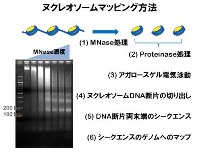
酵母のヌクレオソームマップデータよりヌクレオソームDNAの長さを比較する
Compare the nucleosomal DNA lengths based on the yeast nucleosome mapping data.
Data:
cont1, nuclesomal DNA fragment on chromosome 1 (the first and last positions) of Saccharomyces cerevisiae control
mut1, nucleosome DNA fragment of ELP3 (one of histone acetyltransferase genes) deletion mutant
From Matsumoto et al. (2011) PLoS ONE 6: e16372
1) データのダウンロードDownload cont1 and mut1
2) データのRへの読み込み
Read the two data into R
cont1 <- read.table("cont1")
mut1 <- read.table("mut1")
dim(cont1)
によりデータを確認Confirm the matrix
27963行2列となれば良い
dim(mut1)
こちらは13737行2列となれば良い
3) ヌクレオソームDNA長さの比較
Compare the nucleosomal DNA lengths
cont1L <- cont1[ ,2]-cont1[ ,1]+1
1列目は断片の最初、2列目は最後の位置を示すので、その長さは差に1を足したものとなる、そのデータをcont1Lに収納する
mut1L <- mut1[ ,2]-mut1[ ,1]+1
ELP3欠失株における長さのデータをmut1Lに収納する
range(cont1L); range(mut1L)
データの範囲を確認、92 214および92 235となれば良い
length(cont1L); length(mut1L)
サイズの確認、こちらは先の行数と一致すれば良い
par(mfrow=c(2,1))
hist(cont1L, breaks=seq(90, 240, 1))
hist(mut1L, breaks=seq(90, 240, 1))
90塩基から240塩基の範囲で間隔1のヒストグラムを作成する
数が異なるものの分布を比較したいときにはprob=Tにすると良い
hist(cont1L, breaks=seq(90, 240, 1), prob=T)
hist(mut1L, breaks=seq(90, 240, 1), prob=T)
par(mfrow=c(1,2))
boxplot(cont1L, mut1L)
boxplot(cont1L, mut1L, range=2)
箱ひげ図におけるひげはDefault range=1.5となっている
summary(cont1L); summary(mut1L)
4) データの抽出とその保存Extract and save data
cont1over200 <- cont1[cont1[,2]-cont1[,1]+1>200,]
長さが200塩基を超えるものをcont1over200として収納する
nrow(cont1over200)/nrow(cont1)
は200塩基を超える割合を示す
write.table(cont1over200, "cont1over200.txt", quote=F, row.names=F, col.names=F)
はcont1over200をRからテキストファイルとして書き出す
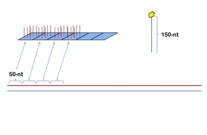
[2-2] 頑強性Robustness
どの代表値を選ぶかWhich representative value is selected?
例えば、ゲノム塩基配列を50塩基毎に区切り、それらの配列を持ったDNAプローブを搭載したマイクロアレイにより150塩基の長さのDNAを検出する。連続する21のプローブのシグナル値がaであった場合、3プローブで一つの代表値を設定する際にそれを中央値あるいは平均値としたときのどれほどの違いが見られるか。なお、11番目の「10」はノイズである。
For example, please image an experiment using the tiling array with 50 bp resolution. When the labeled DNA for the hybridization to the array has 150 nucleotides length, the labeled DNA is detected by 3 or 4 consecutive probes. a, signal intensities of 21 consecutive probes. Which is better mean or median as the representative value in this case? Please consider that the 11th signal intensity (10) is a noise.
a <- c(runif(10),10,runif(10))
d1 <- c()
for(i in 1:length(a)) d1[i] <- median(a[i:(i+2)])
は中央値を代表値として選び、d1に収納するMedian as the representative value
d2 <- c()
for(i in 1:length(a)) d2[i] <- mean(a[i:(i+2)])
は平均値を代表値として選び、d2に収納するMean as the representative value
plot(d1, ylim=c(0,10), ylab="intensity", col="red", type="l")
par(new=T)
plot(d2, ylim=c(0,10), ylab="intensity", col="blue", type="l")
により、青(平均値を代表値とした場合)がノイズの影響をより強く受けることが確認できる
[2-3] サンプルの最大値と最小値の間に母集団の中央値がある確率
Probability that median of a population exits within the rage of a sample
1) 母集団が一様分布、サンプルサイズ3、サンプリング回数1000回の場合
Population, uniform distribution
Sample size, 3
Sampling number, 1000 times
a <- matrix( ,1000, 2)
により1000行2列の行列aを用意するPrepare a matrix of 1000 rows and 2 columns
for(i in 1:1000) a[i, ] <- range(runif(3))
aの1列目に最小値、2列目に最大値を入れる
nrow(a[a[ ,1] < 0.5 & a[ ,2] > 0.5, ])
最小値が0.5未満、最大値が0.5より大きいサンプルの数を数える
理論値は1-2×0.53 = 0.75
2) 母集団が一様分布、サンプルサイズ5、サンプリング回数1000回の場合
Sample size, 5; sampling number, 1000
a <- matrix( ,1000, 2)
for(i in 1:1000) a[i, ] <- range(runif(5))
nrow(a[a[ ,1] < 0.5 & a[ ,2] >= 0.5, ])
理論値は0.9375, n個のデータの場合の理論値は1 – (2 / 2n)
3) サンプルデータの最大値と最小値の間に第一四分位数(下側四分位数)がある確率が0.99以上になる最小のサンプルサイズを求めるには
a <- function(n) 1-(1/4)^n-(3/4)^n
この関数は単調増加Monotonically increasing
b <- a(1:100)
nは整数値であるので、1から100までの様子をプロットする
plot(b)
100-length(b[b >= 0.99])+1
により、0.99以上になる最小のnが求められる
[2-4] ウィルコクソン順位和検定(マン・ホイットニーU検定)Wilcoxon rank sum test (Mann-Whitney U test)
Wilcoxon F (1945) Individual comparisons by ranking methods. Biometrics Bulletin 1, 80-83.
Mann HB, Whitney DR (1947) On a test of whether one of 2 random variables is stochastically larger than the other. Annals of Mathematical Statistics 18, 50-60.
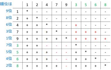
例えば
第一のサンプルデータ: 1, 2, 4, 7, 9
第二のサンプルデータ: 3, 5, 6, 8
これらの母集団に有意な差があるか検定する
Sample #1: 1, 2, 4, 7, 9
Sample #2: 3, 5, 6, 8
Do the two populations have significant difference?
(1) 帰無仮説と対立仮説を決める
帰無仮説: 第一、第二のサンプルの母集団に差がない
対立仮説: 第一、第二のサンプルの母集団に差がある
Null hypothesis: no significant difference
Alternative hypothesis: significant difference
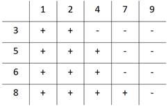
(2) 検定統計量を決めるDetermine test statistic
第二のデータの方が大きいときに「+」、小さいときに「–」と表すと「+」が12で「–」が8である。Uを「+, –」の数の少ない方とすると、U = 8
第一、第二のデータ間において違いが大ききほどUは小さくなる
When the sample #2 element is bigger than the sample #1 element, describe “+”.
When #2 element is smaller than #1 element, describe “–”.
In this case, number of “+” is 12, number of “–” is 8.
The statistic U is defined as the fewer number either the number of “+” or that of “–”.
Thus, U = 8.
The greater the difference is, the smaller the U is.
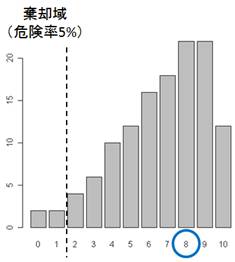
(3) 検定統計量の分布を描く
Describe the distribution of the statistic
帰無仮説に基づくすべてのパターンを考える
1, 2, .., 9から5つを取り出す場合の数は
一回目に取り出せる数字は9通り、二回目は8通り、三回目は7通り、四回目は6通り、五回目は 5 通り
しかし、順番は関係ないので、取り出した5つの並び方5!で割る必要がある
9×8×7×6×5/5! = 126(Rではchoose(9,5))
帰無仮説のもと、これら 126 通りは等確率で生じる
Consider all patterns based on the null hypothesis.
When you extract five elements from the nine elements, at the first time you have nine cases, at the second you have eight cases, ..., at the fifth you have five cases.
However, you do not need to consider the order of extraction.
Thus,
9×8×7×6×5/(5×4×3×2×1) = 126
According to the null hypothesis, these 126 ways happen equally.
126通りのそれぞれについてUを調べると表のようになる
Table of Statistic U, Number of cases, and Probability
|
U |
数 |
確率 |
|
0 |
2 |
0.016 |
|
1 |
2 |
0.016 |
|
2 |
4 |
0.032 |
|
3 |
6 |
0.048 |
|
4 |
10 |
0.079 |
|
5 |
12 |
0.095 |
|
6 |
16 |
0.127 |
|
7 |
18 |
0.142 |
|
8 |
22 |
0.175 |
|
9 |
22 |
0.175 |
|
10 |
12 |
0.095 |
|
計 |
126 |
1 |
(4) 有意水準(危険率)を決める
Significance level = 0.05
(5) データからの検定統計量が棄却域に入るか否かをみる
Investigate whether U of the data locates in rejection region or not.
When U = 8,
p-value = 0.016+0.016+0.032+0.048+0.079+0.095+0.127+0.142+0.175 = 0.73
(6) 棄却域に入った場合、帰無仮説を棄却する
When the statistic locates in rejection region (the p-value < 0.05), you reject the null hypothesis. In this example, we cannot reject the null hypothesis.
a <- c(1, 2, 4, 7, 9)
b <- c(3, 5, 6, 8)
wilcox.test(a, b)
names(wilcox.test(a, b))
wilcox.test(a, b)$statistic
U値
wilcox.test(a, b)$p.value
マン・ホイットニーU検定における「+」の数をUp、「-」の数をUmとし、サンプル1のサンプルサイズN1、順位和Rank sumをR1、サンプル2のサンプルサイズN2、順位和をR2とし、UpおよびUmをN1、N2、R1、R2で示す
順位を数の大きなものからつけた場合
各順位 = (マイナスの数 + 1)となっている(次の表)
自己対戦の部分におけるプラスとマイナスの数は等しく
((N1)2 – N1)/2および((N2)2 – N2)/2
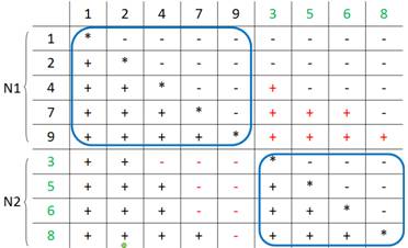
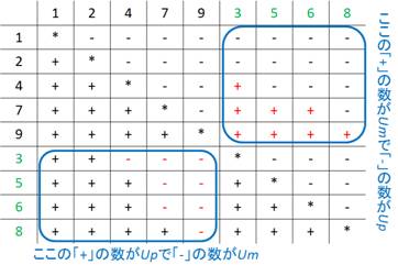
以上より
グループ1の順位和
R1 = ((N1)2 – N1)/2 + Up + N1 = Up + ((N1)2 + N1)/2
∴ Up = R1 - ((N1)2 + N1)/2
同様に R2 = ((N2)2 – N2)/2 + Um + N2 = Um + ((N2)2 + N2)/2
∴ Um = R2 - ((N2)2 + N2)/2
すなわち、順位和からU値を求めることができる
[2-5] t検定t test
Student (1908) The probable error of a mean. Biometrika 6, 1-25.
Student = William Sealy Gosset (1876-1937)
Gossetはギネスビールの社員であったため、ペンネームを使用して論文発表した
Gosset used the pen name “Student” because he was an employee of Guinness
1標本One sample
t = (mean of sample – μ)/{sd of sample/sqrt(sample size)}
平均値の標準誤差Standard error of the mean (SEM)
SEM = σ/sqrt(n)
これはt検定統計量の分母
2標本Two samples
t = difference between sample means/sqrt{(σ of sample #1/ sqrt(sample size #1))2+(σ of sample #2/ sqrt(sample size #2))2}
平均値の差の標準誤差Standard error of difference of means (SEDM)
SEDM = sqrt(SEM12 + SEM22)
a <- c(1, 2, 4, 7, 9)
t.test(a)
One sample t test, default, μ = 0
t.test(a, mu = 4)
When μ = 4, will the null hypothesis reject?
ではどの程度の範囲で棄却されないか?
信頼区間Confidence intervalを調べる
d1 <- seq(1, 9, 0.1)
d2 <- c()
for(i in 1:length(d1)) d2[i] <- t.test(a, mu = d1[i])$p.value
plot(d2)
abline(0.05, 0, col="red")
d2[d2<0.05]
x <- seq(-5, 5, 0.1)
plot(x, dt(x, 4))
は自由度4のt分布の様子を示す
t distribution with degree of freedom, df = 4
qt(0.975, 4)
は棄却境界p = 0.975のxの値
mean(a) + qt(0.975, 4)*sd(a)/sqrt(5)
によりaの場合の信頼区間の上限がわかる
t.test(a)
により信頼区間は示されている
a <- c(1, 2, 4, 7, 9)
b <- c(3, 5, 6, 8)
t.test(a, b)
Two samples t test
t.test(a, b)$statistic
によりt値をだけを示すことができる
(mean(a)-mean(b))/sqrt((sd(a)/sqrt(length(a)))^2+(sd(b)/sqrt(length(b)))^2)
t.test(a, b, var.equal=T)
は等分散を仮定した場合であるAssuming equal variances
var.test(a, b)
により等分散かどうかを調べるTest of equal variances, F test
F 検定
x <- seq(0, 5, 0.01)
plot(x, df(x, 4, 3))
F distribution with df = (4, 3)
var(a)/var(b)
分散の比がF値
当然ながら、var.test(a, b)$p.value = var.test(b, a)$p.value
[2-6] 演習Practice
次のそれぞれの場合において、aとb間におけるウィルコクソン順位和検定およびt検定を行う
Perform the Wilcoxon rank sum test and t test in the following three cases
1)
a <- runif(100)
b <- c(runif(99), 1)
wilcox.test(a, b)
var.test(a, b); t.test(a, b, var.equal=T)
2)
a <- runif(100)
b <- c(runif(99), 10000)
wilcox.test(a, b)
var.test(a, b); t.test(a, b)
3)
a <- runif(100)
b <- c(runif(95), rep(10000, 5))
wilcox.test(a, b)
var.test(a, b); t.test(a, b)