2012�N�x �o�C�I�X�^�e�B�X�e�B�N�X��b�_ �e�L�X�g3
Introduction to Biostatistics 2012, Text 3
���c�m��Hiromi Nishida
�u�`�E���K��:2012�N5��9���i���j
[3-1] ��1��̉ߌ�Ƒ�2��̉ߌ�Type I and type II errors
��1��: �A���������������Ƃ��ɂ�������p
��2��: �A���������Ԉ���Ă���Ƃ��ɂ�����̑�
par(mfrow=c(2, 2))
a <- c()
for(i in 1:1000) a[i] <- t.test(runif(10), runif(10))$p.value
length(a[a<0.05])
������W�c�i�����ł͈�l���z�j����10�̃T���v�����O��Ɨ��ɍs���A������t�����1000��s�������ʂɂ���p�l<0.05�̐��𐔂���
Count the number of p < 0.05
hist(a)
�T���v���T�C�Y��1000�ɂ����ꍇ�ɂ�
for(i in 1:1000) a[i] <- t.test(runif(1000), runif(1000))$p.value
length(a[a<0.05])
hist(a)
��W�c���قȂ�i�����ł͈�l���z�Ɛ��K���z�j�̏ꍇ�ɂ�
for(i in 1:1000) a[i] <- t.test(runif(10), rnorm(10))$p.value
length(a[a<0.05])
hist(a)
�قȂ��W�c�ŃT���v���T�C�Y��1000�ɂ����ꍇ�ɂ�
for(i in 1:1000) a[i] <- t.test(runif(1000), rnorm(1000))$p.value
length(a[a<0.05])
hist(a)
[3-2]���o��Statistical power
�L�Ӑ����i�댯���j���^�̉��������p����m���������A���̒l���������������قǁA�U�̉��������p����Ȃ��ꍇ�������B���o�͂Ƃ͋U�̉��������p�����m���������B�ʏ�A�댯��Significance level=0.05�A���o��=0.8�ƂȂ�W�{�̑傫�����K�v�ƂȂ�
Significance level is the probability that the test rejects the null hypothesis when it is true. On the other hand, statistical power is the probability that the test rejects the null hypothesis when it is false.
�Ⴆ�A���o��0.8�A�L�Ӑ���0.05�A�W����2�̕��z�ɂ�����0.5�̍������肷�邽�߂ɕK�v�ȕW�{�̑傫����
power.t.test(power=0.8, sig.level=0.05, sd=2, delta=0.5)
�ɂ��253�����܂�
�W�{�̑傫�� 200�A�L�Ӑ���0.05�A�W����2�̕��z�ɂ�����0.5�̍������肷��Ƃ��̌��o�͂�
power.t.test(n=200, sig.level=0.05, sd=2, delta=0.5)
�ɂ��0.703�����܂�
�����̔�r:������60������75���ɏ㏸�������Ƃ�80���̌��o�͂Ō��肷�邽�߂̐������߂�ꍇ��
power.prop.test(power=0.8, p1=0.6, p2=0.75)
�ɂ��T���v���T�C�Y152�����܂�
����power.anova.test�Ȃ�
[3-3] �Ή��̂���f�[�^Paired data
�Ⴆ�A9�l������A����ю���B���A���ꂼ��100�_���_�ŕ]������A���̌��ʂ͉��L�̒ʂ�ł�����
Nine persons took the examinations A and B. The scores are following.
Persons #1, #2, #3, #4, #5, #6, #7, #8, #9
Scores of A: 11, 32, 23, 44, 35, 26, 37, 38, 19
Scores of B: 20, 31, 32, 33, 44, 35, 46, 47, 28
����A��B�̓�Փx�ɂ͍����Ȃ��ƌ����邩���肷��
�����̌��ʂ͂��ꂼ��Ή�Paired (Dependent)���Ă���Ɨ�Unpaired (Independent)�ł͂Ȃ��̂�
x <- c(11, 32, 23, 44, 35, 26, 37, 38, 19)
y <- c(20, 31, 32, 33, 44, 35, 46, 47, 28)
t.test(x, y, var.equal=T); wilcox.test(x, y)�Ƃ���̂͊ԈႢ
t.test(x, y, paired=T); wilcox.test(x, y, paired=T)
�Ƃ��Ȃ���Ȃ�Ȃ�
�Ȃ��A������
t.test(x - y); wilcox.test(x - y)
�ɓ�����
1�W�{�̌���ɂ����ẮA�f�t�H���g���� = 0�ƂȂ��Ă��邽��
[3-4] ��A�Ƒ���Regression and correlation
�f�[�^y���f�[�^x�̊��Ƃ��ĕ\�������Ƃ��A���`��A��p���ē�̕ϐ��̊W������Express the relationships between the two variables
���`��A���f��Linear regression model�Ƃ��āAy[i] = a + bx[i] + residual[i]
�Ƃ����ꍇ�A�c�������aSum of residual squared = ��(y[i] – a – bx[i])2 ���ŏ��ɂ���a�Ab�����߂�B����a�Ab��y�ؕЁA�X���Ƃ��钼������A���� Linear regression line�ƌĂ�
lm(y~x)
���`���f��Linear model
y, dependent variable
x, independent variables
summary(lm(y~x))
plot(x,y)
abline(lm(y~x))
fitted(lm(y~x))
�͓��Ă͂ߒlFitted values������
resid(lm(y~x))
�͎c��Residual������
�����lMeasured values�Ɠ��Ă͂ߒl���Ō��сA�c�����������}��
segments(x, fitted(lm(y~x)), x, y)
�c���̕��z�����K���z�ɏ]���Ă��邩�ǂ����̖ڈ��Ƃ���
qqnorm(resid(lm(y~x)))
�Q�l�܂ł�
��(y[i] - a - bx[i])2
= ��y[i]2 + ��a2 + ��b2x[i]2 - 2��ay[i] + 2��abx[i] - 2��bx[i]y[i]
= ��y[i]2 + na2 + b2��x[i]2 - 2a��y[i] + 2ab��x[i] - 2b��x[i]y[i]
a�ŕΔ�������
2na - 2��y[i] + 2b��x[i] = 0
�����
a = (��y[i] - b��x[i])/n
���l��b�ŕΔ�������
2b��x[i]2 + 2a��x[i] - 2��x[i]y[i] = 0
�����
b��x[i]2 + (��x[i]��y[i] - b��x[i]��x[i])/n – ��x[i]y[i] = 0
b(��x[i]2 – ��x[i]��x[i]/n) + ��x[i]��y[i]/n - ��x[i]y[i] = 0
�ȏ���
b = (��x[i]y[i] – ��x[i]y[i]/n)/(��x[i]2 – ��x[i]��x[i]/n)
a = ��y[i]/n – (Sxy/Sxx)��x[i]/n
Sxy = ��x[i]y[i] – ��x[i]y[i]/n
Sxx = ��x[i]2 – ��x[i]��x[i]/n
[3-5] ���W��Correlation coefficient
�s�A�\��Karl Pearson (1857-1936)�̐ϗ����W��
Pearson product-moment correlation coefficient
r = ��((x[i]-x�̕���)(y[i]-y�̕���))/sqrt(��(x[i]-x�̕���)2�E��(y[i]-y�̕���)2)
�X�s�A�}��Charles Edward Spearman (1863-1945)�̏��ʑ��W��
Spearman rank correlation coefficient�ł�x[i]�Ay[i]�����ꂼ��ɂ����鏇�ʂƂȂ�
�P���h�[��Maurice George Kendall (1907-1983)�̏��ʑ��W��
Kendall rank correlation coefficient

(x1 - x2)��(y1 - y2) < 0
(x1 - x3)��(y1 - y3) > 0
n�̃f�[�^���������o���g�ݍ��킹��n(n-1)/2�ʂ肠��A�����̊W�͐��܂��͕��ƂȂ�B���̂Ƃ���1�A���̂Ƃ���-1��^���A���a��n(n-1)/2�Ŋ���ƁA���̂Ƃ��̒l(��)��-1������1�ƂȂ�B���̂Ƃ��������P���h�[���̏��ʑ��W���Ƃ���
���W���Ɋւ��錟��Test for association between paired samples
�A������: ���ւȂ�(���W����0)
Null hypothesis: correlation coefficient = 0
�s�A�\���̐ϗ����W���̗L�Ӑ�����
cor.test(x, y, method="pearson")
method="p"�ł��Adefault
���蓝�v��Statistic: r�~sqrt(n-2)/sqrt(1-r2)
���R�xDegree of freedom n-2��t���z
�X�s�A�}���̏��ʑ��W���̗L�Ӑ�����
cor.test(x, y, method="spearman")
method="s"�ł���
�P���h�[���̏��ʑ��W���̗L�Ӑ�����
cor.test(x, y, method="kendall")
method="k"�ł���
cor(x, y)*sd(y)/sd(x) = ��A�����̌X��Slope of the regression line
�܂��A��A�����͎听������Principal components analysis�̑��听���Ƃ͈قȂ�
[3-3]��x�Ay�Ŋm�F
prcomp(data.frame(x, y))
summary(prcomp(data.frame(x, y)))
[3-6] ���K�k�N���I�\�[���ʒu�̕ۑ��x��rComparison between nucleosome position profiles
�o��y��q�X�g���A�Z�`�����y�fElp3���k�N���I�\�[���̈ʒu�ɗ^����e���ׂ邽�߁A���̈�`�q�������̃k�N���I�\�[���}�b�v���R���g���[���Ɣ�r����B�{���K�ł͑����F�̂̈�`�q�ɂ�����v�����[�^�̈�i�|��J�n�㗬1000����̈�j����у{�f�B�̈�i�|��J�n����I���܂ł̗̈�j�̃k�N���I�\�[���}�b�v���r����B
In order to elucidate the influence of the histone acetyltransferase Elp3 on positions of nucleosomes, compare two nulceosome maps of control and the ELP3 deletion mutant of Saccharomyces cerevisiae. In this practice, we compare the nucleosome maps in the gene promoter (region from 1 kb upstream of the translational start site) and in the gene body (region from the translational start site to the end) of genes on the chromosome 1.
1) �f�[�^�̃_�E�����[�hDownload data and executable statements
2) �f�[�^��R�ւ̓ǂݎ��Read the data into R
a <- read.table("cont1.txt")
A <- read.table("mut1.txt")
chr1p <- read.table("chr1p.txt")
3) ��r����͈́i����ʒu�j�����߂�Determine the region on the chromosome
x <- chr1p[1, 1]
y <- chr1p[1, 2]
4) �f�[�^�𒊏o����Extract the data in the region
a1 <- a[a[,1]>=x & a[,2]<=y, ]
5) �f�[�^������Arrange the extracted data
a2 <- data.frame(a1[,1]-x+1, a1[,2]-x+1)
a3 <- y-x+1
b <- numeric(nrow(a2)*a3)
for(i in 1:nrow(a2)) b[seq(a3*i+a2[i,1]-a3, a3*i+a2[i,2]-a3)] <- 1
b1 <- matrix(b, nrow=nrow(a2), byrow=T)
b2 <- apply(b1, 2, sum)
6) �v���t�@�C�����m�F����Confirm the data
plot(b2, type="h")
7) 4)�Ɠ������Ƃ�ψي��ł��s��Do the same operation for the mut1
A1 <- A[A[,1]>=x & A[,2]<=y, ]
A2 <- data.frame(A1[,1]-x+1, A1[,2]-x+1)
B <- numeric(nrow(A2)*a3)
for(i in 1:nrow(A2)) B[seq(a3*i+A2[i,1]-a3, a3*i+A2[i,2]-a3)] <- 1
B1 <- matrix(B, nrow=nrow(A2), byrow=T)
B2 <- apply(B1, 2, sum)
8) �R���g���[���ƕψي��̃v���t�@�C�����r����Compare between the control and the mutant
plot(b2, type="l", ylim=c(0,50), xlab="", ylab="")
par(new=T)
plot(B2, type="l", ylim=c(0, 50), col="blue", xlab="", ylab="")
9) ���W�����v�Z����Calculate the correlation coefficient
cor(b2, B2)
10) Identify nucleosome free region and exclude the region. [�e�̈�̃k�N���I�\�[���̐����J�E���g]
source("R_count.txt")
11) 10)�̌��ʂɂ����Đ����[���̗̈�ׂ�
D[D[,1]==0 | D[,2]==0 | D[,3]==0 | D[,4]==0,]
12) �[���̗̈���������̈悾����ΏۂƂ���
chr1p <- chr1p[c(1:15, 17:34, 36:38, 41:45, 47:66, 68:78, 80:94),]
chr1b <- chr1b[c(1:15, 17:34, 36:38, 41:45, 47:66, 68:78, 80:94),]
13) 3)����9)�̑�������ׂĂ̈�`�q�ɂ��čs��Execute R_Chr1_pro.txt
source("R_Chr1_pro.txt")
14) ���W���̕��z�̗l�q������Distribution of the correlation coefficients
hist(datapro)
boxplot(datapro)
15) 13)�Ɠ��l�ɂ���databod���쐬����Execute R_Chr1_bod.txt
source("R_Chr1_bod.txt")
16) �e��`�q�̃v�����[�^�̈您��у{�f�B�̈�̑��W�����r����Compare the correlation coefficients between datapro and databod
DATA <- data.frame(datapro, databod)
boxplot(DATA)
matplot(DATA, type="b", ylab="Correlation", xlab="gene")
matplot(t(DATA), type="l", xaxt="n", xlab="Region", ylab="Correlation"); axis(1, c(1, 2), c("Promoter", "Body"))
nrow(DATA[DATA[,1] > DATA[,2], ])
nrow(DATA[DATA[,1] < DATA[,2], ])
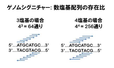
[3-7] ���K�Q�m���V�O�j�`���[��rComparison of genome signatures
Data: gs.txt�i�A������ 2 ����̊e�Q�m�� DNA �ɂ�����o���p�x�f�[�^�j
Ecoli, Escherichia coli; Bsublitis, Bacillus subtilis; Mgenitalium, Mycoplasma genitalium; Sgriseus, Streptomyces griseus
1) �f�[�^�̃_�E�����[�hDownload gs.txt
2) �f�[�^��R�ւ̓ǂݍ���Read the two data into R
gs <- read.table("gs.txt")
3) Ecoli��Bsubtilis�̃Q�m���V�O�j�`���[�̑��W�����o��
cor(gs$Ecoli, gs$Bsubtilis)
4) ���ׂĂ̐����Ԃ̃Q�m���V�O�j�`���[�̑��W�����o��
cor(gs)
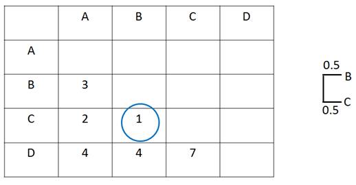
[3-8] �K�w�I�N���X�^�����OHierarchical clustering
���[3-3]�̐��l�ω����f�[�^�t���[����
x <- c(11, 32, 23, 44, 35, 26, 37, 38, 19)
y <- c(20, 31, 32, 33, 44, 35, 46, 47, 28)
d <- data.frame(x, y)
plot(d)
�e�|�C���g�Ԃ̋��������߂�
dist(d)
Distance matrix computed by using the Euclidean distance measure to compute the distances between the rows of the data matrix
�����f�[�^�Ɋ�Â��K�w�I�N���X�^�����O
plot(hclust(dist(d)))
Hierarchical clustering
�U�z�}�ƃN���X�^�����O���r�����
par(mfrow=c(1, 2))
plot(d, pch=c("1", "2", "3", "4", "5", "6", "7", "8", "9")); plot(hclust(dist(d)))
[3-7]�Ɋ�Â�����2�̃N���X�^�����O���r
plot(hclust(dist(gs)))
plot(hclust(dist(t(gs))))
heatmap(as.matrix(gs))
���ϘA���@Unweighted pair-group method using arithmetic averages
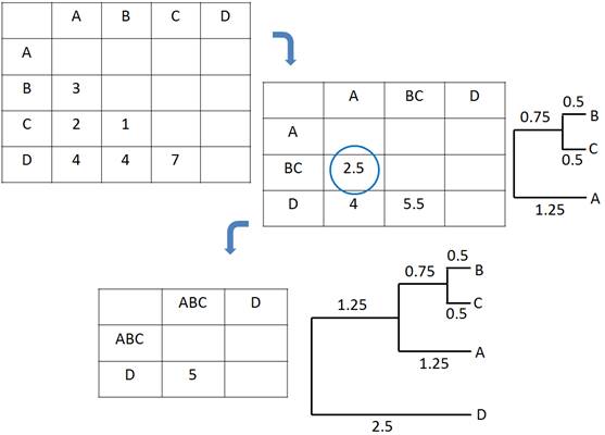
��K�w�I�N���X�^�����O
data <- kmeans(as.matrix(data.frame(x, y)), 3)
plot(data.frame(x, y), col=data$cluster)
points(data$centers, col=1:3, pch=4)
[3-9] �R�����S���t�E�X�~���m�t����Kolmogorov-Smirnov test
�ݐϑ��Γx�����z��r�ɂ�錟��
Test based on cumulative relative frequency distribution comparison
Andrey Nikolaevich Kolmogorov (1903–1987)
Nikolay Vasilyevich Smirnov (1900–1966)
1)�ݐϊm�����zCumulative probability distribution
x <- seq(-5, 5, 0.1)
y1 <- dnorm(x)
�m�����x���lProbability density function
y2 <- pnorm(x)
�ݐϊm�����z���l
par(mfrow=c(2, 2))
plot(x, y1); plot(x, y2)
Y1 <- dunif(x, -5, 5)
Y2 <- punif(x, -5, 5)
plot(x, Y1); plot(x, Y2)
2)�R�����S���t�E�X�~���m�t����Kolmogorov-Smirnov test
u <- runif(50)
50 random numbers from a uniform distribution (in the range from 0 to 1)
mean(u)
Nearly 0.5
n <- rnorm(50, 0.5)
50 random numbers from a normal distribution (mean=0.5, sd=1)
mean(n)
Nearly 0.5
par(mfrow=c(2,1))
hist(u); hist(n)
Different distributions
var.test(u, n)
Different variances
t.test(u, n)
t test
wilcox.test(u, n)
Wilcoxon rank sum test
ks.test(u, n)
Kolmogorov-Smirnov test