2012年度 バイオスタティスティクス基礎論 テキスト4
Introduction to Biostatistics 2012, Text 4
西田洋巳Hiromi Nishida
講義・実習日:2012年5月16日(水)
[4-1] 分散分析ANOVA, Analysis of variance
|
Group |
A |
B |
C |
|
|
2 |
1 |
2 |
|
|
4 |
3 |
3 |
|
|
9 |
5 |
4 |
|
|
|
7 |
|
|
Mean |
5 |
4 |
3 |
総平方和Total sum of squares (SS)=グループ間平方和SS between groups+グループ内平方和SS within group
(2-4)2+(4-4)2+(9-4)2+(1-4)2+(3-4)2+(5-4)2+(7-4)2+(2-4)2+(3-4)2+(4-4)2=54
(5-4)2+(5-4)2+(5-4)2+(4-4)2+(4-4)2+(4-4)2+(4-4)2+(3-4)2+(3-4)2+(3-4)2=6
(2-5)2+(4-5)2+(9-5)2+(1-4)2+(3-4)2+(5-4)2+(7-4)2+(2-3)2+(3-3)2+(4-3)2=48
群別平均値の有意な差を見出すための検定は、2つの分散の推定値比較によってなされる
|
Source |
SS |
自由度df |
平均平方Mean square |
F value |
|
Group |
6 |
3-1=2 |
6/2=3 |
3/6.8=0.44 |
|
Error |
48 |
10-3=7 |
48/7=6.8 |
|
|
Total |
54 |
10-1=9 |
F distribution with df = (2,7)
x <- seq(0, 10, 0.05)
y <- df(x, 2, 7)
plot(x, y)
一元配置分散分析One way ANOVA
a1 <- c(2, 4, 9); a2 <- c(1, 3, 5, 7); a3 <- c(2, 3, 4)
data <- c(a1, a2, a3)
group <- factor(rep(1:3, c(3, 4, 3)))
Not numerical but factor
anova(lm(data~group))
分散分析表ANOVA tableの出力
oneway.test(data~group)
一元配置分散分析
oneway.test(data~group, var.equal=T)
等分散を仮定Assuming equal variances
bartlett.test(data~group)
等分散の検定Test of equal variances
kruskal.test(data~group)
クラスカル・ウォリス検定Kruskal-Wallis test
データの順位に基づき検定
Kruskal WH, Wallis WA (1952) Use of ranks in one-criterion variance analysis. Journal of the American Statistical Association 47, 583-621.
Parametric statistical tests:
t.test, var.test, oneway.test, bartlett.test
Nonparametric tests:
wilcox.test, kruskal.test, ks.test
どの群間に差があるかを調べる場合
a <- c(1, 2, 3, 4, 5, 6, 7, 8, 10)
b <- factor(c(1, 1, 1, 2, 2, 2, 3, 3, 3))
bartlett.test(a~b)
等分散の確認
oneway.test(a~b, var.equal=T)
pairwise.t.test(a, b)
pairwise.t.test(a, b, pool.sd=F)
共通の標準偏差を用いない場合
pairwise.t.test(a, b, pool.sd=F, p.adj="bonf")
Holm補正からBonferroni補正へ
t.test(c(1, 2, 3), c(7, 8, 10))$p.value
t.test(c(4, 5, 6), c(7, 8, 10))$p.value
t.test(c(1, 2, 3), c(4, 5, 6))$p.value
との比較からHolmおよびBonferroni補正を確認
二元配置分散分析Two way ANOVA
酵母の遺伝子の数が染色体およびDNA鎖で偏りがあるか
Saccharomyces cerevisiae has 16 chromosomes. Number of genes on the Watson strand (which has 5’-end at the short-arm telomere) from the chromosome #1 to #16 are 51, 187, 68, 371, 137, 64, 275, 153, 94, 183, 159, 244, 240, 206, 278, and 244, respectively. Number of genes on the Click strand from the chromosome #1 to #16 are 46, 219, 90, 377, 136, 62, 250, 128, 111, 173, 151, 268, 221, 187, 258, and 216, respectively.
watson <- c(51,187,68,371,137,64,275,153,94,183,159,244,240,206,278,244)
click <- c(46,219,90,377,136,62,250,128,111,173,151,268,221,187,258,216)
matplot(data.frame(watson, click), type="b")
data <- c(watson, click)
wc <- factor(c(rep(1, 16), rep(2, 16)))
chr <- factor(rep(1:16, 2))
anova(lm(data~wc+chr))
ANOVA table
data~chr+wcとしても結果は同じ
par(mfrow=c(2, 1))
interaction.plot(chr, wc, data)
interaction.plot(wc, chr, data)
データフレームからベクトルへの変換を行う
行列として認識させるためには
is.matrix(data.frame(watson, click))
Is it matrix?
data_matrix <- as.matrix(data.frame(watson, click))
is.vector(data_matrix)
data_vector <- as.vector(data_matrix)
anova(lm(data_vector~wc+chr))
Lengths of chr #1 to #16, 230 kbp, 813 kbp, 317 kbp, 1532 kbp, 577 kbp, 270 kbp, 1091 kbp, 563 kbp, 440 kbp, 746 kbp, 667 kbp, 1078 kbp, 924 kbp, 784 kbp, 1091 kbp, and 948 kbp
遺伝子密度に偏りはあるか調べると
size <- c(230, 813, 317, 1532, 577, 270, 1091, 563, 440, 746, 667, 1078, 924, 784, 1091, 948)
data <- c(size/watson, size/click)
anova(lm(data~wc+chr))
[4-2] ニ項検定Binomial test
例えば、ある地域よりサンプリングしたある生物のオスが7匹、メスが1匹であった。これは母集団が性比1:1から有意に差があるといえるか?
5%の危険率で検定せよ
A sample has 7 males and 1 female. Does the population have significant difference from male:female = 1:1?
帰無仮説: 母集団での性比は1:1である
対立仮説: 母集団での性比は1:1でない
Null hypothesis: no significant difference
Alternative hypothesis: significant difference
8匹の性別のパターンは28 = 256通りあり、帰無仮説のもとでは、それぞれが同じ確率1/256で生じる
8匹の中でオスがk匹である場合は(8!/k!/(8-k)!)通り
Consider all patterns based on the null hypothesis.
According to the null hypothesis, 28 = 256 ways happen equally.
In this case, the statistic is defined as the larger number either the number of males or females.
検定統計量をオス・メスの多い方の数とすると
|
Number of males |
Number of females |
Number of cases |
Statistic |
|
8 |
0 |
1 |
8 |
|
7 |
1 |
8 |
7 |
|
6 |
2 |
28 |
6 |
|
5 |
3 |
56 |
5 |
|
4 |
4 |
70 |
4 |
|
3 |
5 |
56 |
5 |
|
2 |
6 |
28 |
6 |
|
1 |
7 |
8 |
7 |
|
0 |
8 |
1 |
8 |
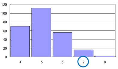
Distribution of the statistic
分布は上図のようになる
p-value = (2 + 16) / 256 = 0.0703125
よって、5%危険率で帰無仮説を棄却できない
Thus, we cannot reject the null hypothesis.
binom.test(1, 8)
Default probability = 0.5
binom.test(1, 8, 0.4)
Probability = 0.4 (ratio of female)の場合
binom.test(2, 16)
binom.test(3, 24)
prop.test(1, 8)
比率の検定Proportion test
prop.test(1, 8, correct=F)
Without continuity correction 連続性の補正、Yatesの補正
prop.test(1, 8, 0.4)
prop.test(c(1, 2), c(1, 8))
2群間Two samplesの比率の差の検定
[4-3] 一般化線形モデルGeneralized linear model
例えば、ある昆虫の性比を国Aで調査ところ4サンプルで(メスの数female 7、オスの数 male 3)、(メスの数20、オスの数30)、 (メスの数50、オスの数150)、(メスの数100、オスの数350)であった。同様に国Bで調査したところ(メスの数8、オスの数2)、(メスの数25、オスの数30)、(メスの数40、オスの数120)、(メスの数90、オスの数300)であった。集団における性比が集団の大きさ、国に関係しているかどうか調べる
Sample #1 (7 females and 3 males), #2 (20 females and 30 males), #3 (50 females and 150 males), and #4 (100 females and 350 males) in the country “A”. Sample #1 (8 females and 2 males), #2 (25 females and 30 males), #3 (40 females and 120 males), and #4 (90 females and 300 males) in the country “B”. Does the sample size or the country influence the sex ratio?
country <- c(rep("A", 4), rep("B", 4))
female <- c(7, 20, 50, 100, 8, 25, 40, 90)
male <- c(3, 30, 150, 350, 2, 30, 120, 300)
size <- female+male
data.frame(country, size, female, male)
summary(glm(cbind(female, male) ~ size * country, binomial))
sizeをlog(size)にした場合の残差逸脱度Residual devianceを比較する
[4-4] フィッシャーの正確確率検定Fisher’s exact probability test
Ronald Aylmer Fisher (1890-1962)
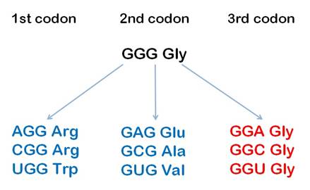
例えば、あるオルソログ遺伝子の塩基置換を生物A、Bにおいて比較したところ、同義的塩基置換サイト99、非同義的塩基置換サイト387、同義的非置換塩基サイト94、非同義的非置換塩基サイト323であった。この場合、同義的・非同義的塩基置換の頻度に有意な差があるといえるか?
When we compared nucleotide substitutions of orthologous genes between organisms “A” and “B”, we found 99 synonymous and 387 nonsynonymous sites in the substitution sites, 94 synonymous and 323 nonsynonymous sites in the nonsubstitution sites.
帰無仮説: 同義的・非同義的塩基置換の頻度は同じ
対立仮説: 同義的・非同義的塩基置換の頻度は同じではない
Null hypothesis: no significant difference of the synonymous/nonsynonymous ratio between the substitution and nonsubstitution sites.
Alternative hypothesis: significant difference.
2×2分割表を作成する
|
Substitution sites |
Nonsubstitution sites |
Total |
|
|
Synonymous |
99 |
94 |
193 |
|
Nonsynonymous |
387 |
323 |
710 |
|
Total |
486 |
417 |
903 |
帰無仮説のもと、この分割表が得られる確率を求める
Total: 903を193と710に分ける場合の数で903!/193!/710!
Substitution sites: 486を99と387に分ける場合の数で 486!/99!/387!
Nonsubstitution sites: 417を94と323に分ける場合の数で 417!/94!/323!
よって(486!/99!/387!)×(417!/94!/323!)/(903!/193!/710!)
さらに、これより極端なものを全て計算し、それらを足し合わせる
a <- matrix(c(99, 94, 387, 323), 2, byrow=T)
fisher.test(a)
[4-5] χ2検定chi (χ) square test
Karl Pearson (1857-1936)
(要素 - 期待値)2/期待値 = χ2
[4-4]の場合
帰無仮説に基づくと、Substitution sitesにおいては
Synonymous 486×193/903、Nonsynonymous 486×710/903
Nonsubstitution sitesにおいては
Synonymous 417×193/903、Nonsynonymous 417×710/903
が期待値である
これらの期待値に基づき、それぞれのχ2を求めることができ、それらの和0.6298を得ることができる
[4-4]場合は自由度1((2-1)*(2-1))のχ2分布を考える
chisq.test(a)
chisq.test(a, correct=F)
連続性の補正(修正)なし、上記の χ2 の値はこの場合
[4-6] 演習
大腸菌A株は5303遺伝子をコードし、そのうち999遺伝子を水平伝播により獲得したと考えられている。また、B株は4278遺伝子を有し、そのうち721遺伝子を水平伝播により獲得したと考えられている
E. coli strain “A” has 5303 genes. 999 of the 5303 genes had been gained by horizontal gene transfer. Strain “B” has 4278 genes. 721 of the 4278 genes had been gained by horizontal gene transfer. Do those strains have a significant different ratio of horizontally transferred genes?
1) 水平移動してきた遺伝子の数に株間で偏りがあるかをχ2 test
chisq.test(matrix(c(999, 721, 5303-999, 4278-721), 2))$p.value
2) Fisher’s exact probability test
fisher.test(matrix(c(999, 721, 5303-999, 4278-721), 2))$p.value
3) χ2検定において、B株における水平伝播した遺伝子数がどの範囲であれば、5%の危険率で有意差なしとなるかを調べる
Calculate the range of number of horizontally transferred genes of strain B, with p-value > 0.05 in the result of the χ2 test
a <- c()
for(i in 1:4277) a[i] <- chisq.test(matrix(c(999, i, 5303-999, 4278-i), 2))$p.value
plot(a)
b <- data.frame(1:4277, a)
range(b[b[,2] > 0.05,][,1])
[4-7] 演習
ゲノムDNAはA-T、G-Cがそれぞれペアを形成し二重螺旋構造をとっている。 あるバクテリアのゲノムは3,000,000塩基対から成り立ち、そのA-Tペアの割合は40%である
The DNA double helix is stabilized by hydrogen bonds between the bases (A-T and G-C pairs) attached to the two strands. One bacterium has a genome DNA (3,000,000 bp), which consists of 1,200,000 A-T pairs (1,800,000 G-C pairs).
1) そのゲノムの一部領域を調べたところ、1000塩基対から成り立ち、A-Tペアの割合が500塩基対であった。この領域の塩基組成は有意に偏っているといえるか
One sequential region of the genome has 1000 bp, which consists of 500 A-T pairs (500 G-C pairs). Does this region have a significant different base composition?
fisher.test(matrix(c(500, 500, 1200000-500, 1800000-500), 2))$p.value
chisq.test(matrix(c(500, 500, 1200000-500, 1800000-500), 2))$p.value
2) 連続する1000塩基対中、何塩基対がA-Tペアであれば、χ2検定においてp値 > 0.05となるか
Calculate the range of number of A-T pairs of 1000 bp, with p-value > 0.05 in the result of the Pearson’s Chi squared test.
a <- c()
for(i in 1:999) a[i]<-chisq.test(matrix(c(i,1000-i,1200000-i,1800000-1000+i),2))$p.value
b <- data.frame(1:999, a)
range(b[b[,2] > 0.05, 1])